


As we enter 2021, active learning is perhaps the least understood and most underutilized technique in machine learning today. Its promise is simple and elegant: to reduce the overall records you use to train models without trading off accuracy. It’s an iterative, incremental process that oscillates between training and inference so that instead of a training your models on large batches of data, you train with smaller subsets of that same data, check your model’s progress between loops, and provide a different subset of your training data.
A key part of any active learning implementation is how you choose those different subsets of data. This is known as your querying strategy. There are myriad ways to do this and we spend a lot of time here at Alectio testing, combining, and tweaking these strategies, though for the sake of this blog, we’re going to stick with two fairly common ones: least confidence and highest entropy. We’ll explain both as we dig in a little deeper.
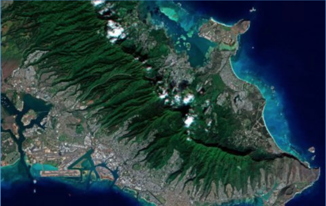
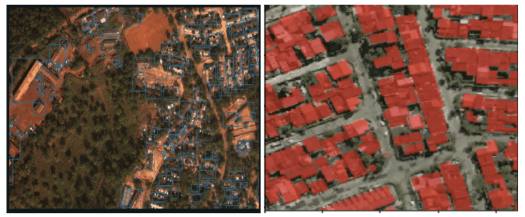
The experiment we’re recapping today concerns aerial imagery and whether an active learning approach can reduce the amount of data we’d need for our models to converge (and thus, the amount of labels we’d need to pay for as well!). We’ll be looking at two different open source aerial imagery datasets: xView and the SpaceNet Challenge I. xView is an object detection data set with more than 60 classes but only 846 images. SpaceNet, meanwhile, is a semantic segmentation set of buildings. Here’s an example of each:

Can active learning reduce the amount of data we need to get high performing models? Let’s find out:
Our experiment
Our goal here is fairly simple: we’d like to determine if actively choosing the data we train our model outperforms randomly choosing data. Since many machine learning projects use all the labeled training data they have, our goal is to see at what point(s) actively choosing data yields better results. We’d like to reach the same level of accuracy with a fraction of the data as typical approaches would get with the entire dataset. In the real world, this would reduce labeling costs as well as compute and storage costs but, of course, these are fully labeled open source datasets we’re working on here.
As mentioned, in active learning, you do not train a model with all your data but with smaller batches of it, selected based on your querying strategy. Here’s how that broke down in these experiments:
- xView: 7 loops with 100 records per loop (700 images)
- SpaceNet: 10 loops with 450 records per loop (4858 images)
In other words, for xView, we first train the model on a random collection of 100 images (that’s because we cannot have a querying strategy based on model performance if the model has yet to be trained at all). Once each loop is done, we’ll use our querying strategy to select the next 100 records our model will be trained on. For example, a least confidence strategy means we’ll be selecting records our model is least confident about.
Last note before we dig into the results: we broke the xView dataset into two separate versions here. Version 1 (v1) is as we described in our intro: a 746 image dataset with 60 unique classes. Our second version (v2) looks at super-classes instead––meaning that all different types of cars would simply be treated as “cars,” for example––so is a 746 image dataset with just 6 classes.
Without further ado, let’s dig into the results:
What we discovered
We’ll start with the xView v1 dataset, the one with 60 unique classes. Below, you’ll see a plot where random sampling is in light purple, high entropy in dark purple, and least confidence in blue. Each hundred-record increment is another loop. Remember that the first 100 are random, but then the next hundred are selected based on the querying strategies we’re testing in this experiment.

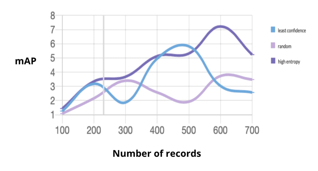
A plot of our first experiment. Mean average precision (mAP) score is x100.
The result above is quite good. It tells us that high entropy-based sampling of 300 records is equivalent to random sampling of 700 records. That’s a reduction of more than half for the same performance.
Now, let’s pause and look at what that would mean in the real world. This is a dataset with less than 800 images but more than a million annotations. That means, on average, we’re looking at savings of more than 470,000 bounding boxes. That’s a lot of bounding boxes. And if you’re familiar with what each of those boxes costs, you can see why this approach might really help keep your budgets reasonable.
Let’s take a look at xView v2 now. This is the simplified dataset with only six classes. Here, random is dark purple, highest entropy is light purple, and least confidence is in blue:

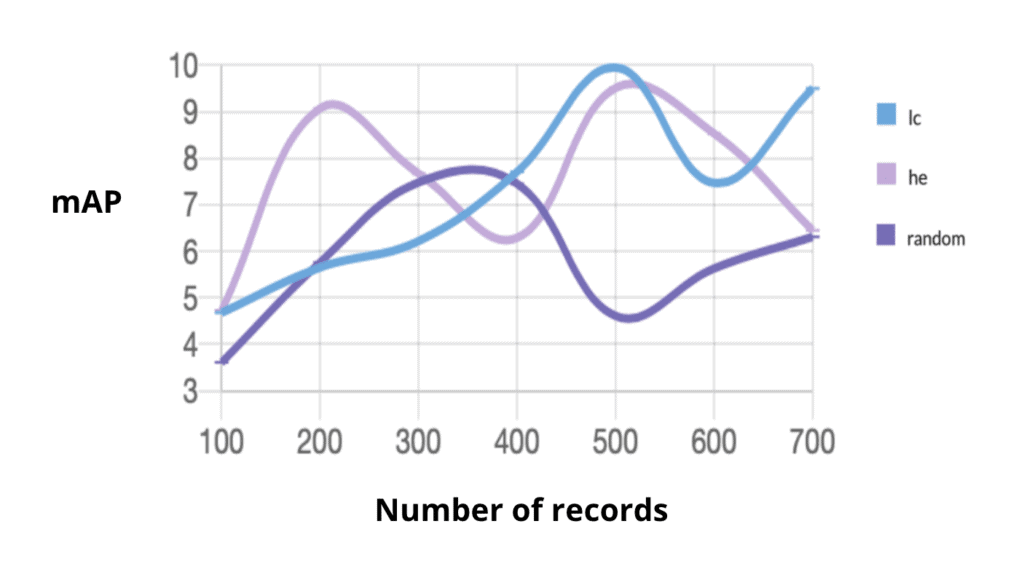
A plot of our experiment on the simplified classes version of xView. Mean average precision (mAP) score is x100
Here, we again see both methods outperforming randomness. In fact, high entropy converges after just 200 records and is only surpassed by selecting 500 records using the least confidence query strategy.
Taken together, these two graphs do underscore something important: choosing a querying strategy is an admittedly difficult and nuanced task. At Alectio, our method is a combination of many different querying strategies. We “listen” to what you model wants and what we select for training evolves as your model learns. Effectively, that means we use an evolving, hybrid querying paradigm that changes at each loop as we adapt to your model’s in-the-moment needs. And, while this might all seem easy once you know which querying strategy works, in reality, it’s rarely feasible to brute-force your way to finding the right one for the right moment. In fact, we don’t think in the normal amount of defined querying strategies, but rather combine and weigh different strategies, counterbalancing them to create an in-the-moment strategy that will be most effective for that loop.
Now, let’s take a look at our other dataset. Here, we’re also testing a minimum margin strategy in addition to the two we used on the xView example. Remember, SpaceNet is a semantic segmentation dataset of just one class: buildings.
The active-learning based improvements on this new dataset are a little harder to see. That’s because the regular training loop converges very quickly (even without any pre-training). But that doesn’t mean there still aren’t exciting findings here.
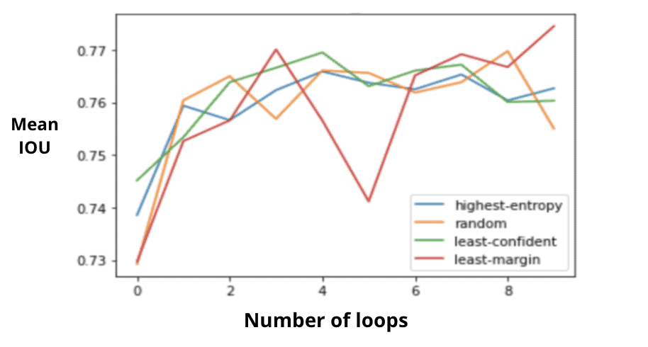

Here, we’re looking at a specific metric for semantic segmentation, mean_iou. “IOU” here stands for “intersection over union” and is defined as “the ratio of intersection of ground truth and predicted segmentation outputs over their union.” Put simply, that basically means how close are our predicted outputs to the ground truth, or, put even more simply, how close did we come to predicting where the buildings are.
A least margin strategy on loop three gives us better performance than a random sampling throughout. In fact, random sampling only gets close to that by loop 8. Broken down into real world labeling costs? That’s more than 2200 images, or about half our dataset here.
Conclusion
We believe one of the most pervasive issues with machine learning today is that bias towards bigger and bigger datasets. It’s contributing to run-away costs and machine learning projects that don’t bring positive ROI to our companies. By reducing the amount of data you need to get your models to converge, you can cut down on all the attendant costs, from labeling to storage to compute.
It’s our goal here at Alectio is to help you find the best data to train your models on and we think that active learning is the key ingredient to making that happen. Using simple, static querying strategies brought us a lot of success that would translate into massive savings in data labeling costs on real world aerial imagery tasks. Using more nuanced, evolving strategies helps even more. And if these results are ones you’d like to replicate for your use case, be it aerial imagery or something else, please do let us know. We’d love to help you get started.