Or how to make Active Learning truly appealing to the industry.
If you are a Data-Centric AI aficionado, the growing interest from the Machine Learning community for Active Learning in the past 18 months should definitely feel very exciting to you. While it had been in existence for several decades, the approach had until recent days been regarded as little more than an obscure Machine Learning technique occasionally used in Academia as a topic of fundamental research. Even the excellent 2009 Active Learning Literature Survey by Burr Settles – probably the most notable attempt to date to popularize Active Learning – had not been enough to attract significant attention to the topic.
We had to wait for the 2020s for the industry to finally begin to grasp the full potential of Active Learning, and it is perhaps a fair question to ask “why now” – or, more accurately, why not earlier?
This is what we will discuss in this post.
Remind me: what is Active Learning again?
If you are not familiar with Active Learning, no worries, you will grasp it very quickly. Otherwise, feel free to skip to the next section.
Like all semi-supervised learning techniques, Active Learning is meant to learn from partially labeled data. What makes it unique is that it is designed to iteratively identify and select the most impactful records within a pool of unlabeled data. It was originally invented in order to reduce labeling costs.
The Active Learning workflow is relatively simple to understand, though building an MLOps pipeline to support it can be a bit more difficult to successfully implement.
It all starts with an initial pool of unlabeled data out of which some records are to be picked and annotated to construct a proper (annotated) training dataset.
The workflow itself is an iteration of the following 4 steps:
- SELECT: some of the data from the initial pool gets selected (“how” it is selected is controlled by a “querying strategy”)
- LABEL: the newly selected data gets annotated and set aside as training data
- TRAIN: the ML algorithm is trained with the selected data (usually, all the data that has been selected so far)
- INFER: the resulting model is used to infer on the data that remains unselected up to that point. The output of that process is used next as an input in the next SELECT step.
The issue with Active Learning, is that it still suffers from the popular perception that its sole function is to keep labeling costs under control (which, as we have discussed elsewhere, is not the case). That reputation led those working in overcapitalized areas of ML (such as autonomous driving) to believe that they could get away with large labeling bills and do away with Active Learning altogether. To researchers in that space and others, Active Learning was just an ancient technique that had since inception been leapfrogged and obsoleted by, among others, Transfer Learning and Self-Learning.
Luckily, the Data-Centric AI movement has rejuvenated interest in the topic, and we can expect a lot of exciting applications to see the light of day in the very near future as a result.
Why is Active Learning so Compute-Heavy?
All that being said, the one aspect that Active Learning legitimately deserves some bad press for is the fact that it can be very computationally expensive.
Going back to the workflow in the previous section, it is easy to see why: while Active Learning is focused on reducing the quantity of necessary labels, it pays no attention to the potential increase in computing caused by repetitive training and additional inference calls. In short, Active Learning tends to be computationally expensive for two reasons:
- The fact that it requires retraining on the same data multiple times. When selecting additional data for the next loop, it is usually assumed that the model will be retrained on the totality of all records selected and annotated so far, not only the ones that were just selected. This leads to the training costs growing quadratically with the amount of data selected.
- The fact that selecting data requires inferring on the unselected data. This means that for a dataset of size 100,000 records and a loop size of 1,000, 99,000 inference calls have to be made. Additionally, because all remaining data is usually considered a candidate for the next loop, most data will be inferred many times before making it into the selected data pool – if at all.
How to Achieve Compute-Efficient Active Learning Processes?
As seen in the previous section, setting up Active Learning in a way that it maximizes savings on labeling can easily lead to breaking the bank from a compute perspective – especially if training on the Cloud. Therefore, before Active Learning can become a truly useful tool for the ML practitioners to manage their operations costs, there is a fundamental need to think about Active Learning as a tradeoff between labeling costs and training costs. Academic papers on Active Learning have long touted a reduction in the quantity of labels in the single digits without even mentioning the explosion in the amount of compute associated with it.
A lot of progress can be made towards a compute-efficient version of Active Learning. Below is a list of how Alectio is keeping Active Learning cost- and compute-efficient, and how you can, too!
By knowing when it’s time to stop
Most Active Learning papers study how to get the most reduction in labeling costs without impacting the performance of the model. This means that researchers run Active Learning processes all the way through in order to prove that their models would have gotten to the same (or a similar) performance with only a certain fraction of the data. Needless to say that repeated trainings and inference cycles lead to unquestionably higher compute bills, because keeping those costs under control was never the target of such research.
In the Industry, though, it only makes sense to adopt Active Learning if the sum of all operational costs (annotations + compute) is worth the trouble. This is only achievable if the Active Learning process is halted before the end – and hopefully at the right time when the learning curve plateaus and that additional data does not benefit the model’s performance anymore.
Now, how can one decide if it’s time to stop before seeing the learning curve flatten and spending money (both for annotations and compute) unnecessarily. The most simple way is to have the ML scientist monitor the process and manually halt. More sophisticated ways involved closely monitoring the loss function or evaluating information density (or lack thereof) at training time.
TL; DR: Just stop the Active Learning process when it stops benefitting your model’s performance.
By avoiding false starts
Some Active Learning research papers (especially those involving classic Machine Learning algorithms) have shown that a poor initialization of the process can stall learning. This could happen for example when the initial selection (which is usually done by random sampling) puts the model in an unrecoverable state such as a deep local minimum. Under such circumstances, any further Active Learning loops would lead to a complete loss of compute, since the training process will not converge anyways. Identifying such stalls can again be done by closely monitoring the evolution of the performance of the model, and aborting the process as early as possible.
TL; DR: If the Active Learning process doesn’t look promising, be ready to stop and reinitialize to avoid wasting compute.
By getting the loop sizes right
When starting out with Active Learning, most practitioners assume that both the querying strategy (the logic used to select the batch of data for the next cycle, or “loop”) and the amount of selected data (the “size” of the loop) have to be predetermined and fixed throughout the entire training process. However, this is not true, though obviously more convenient.
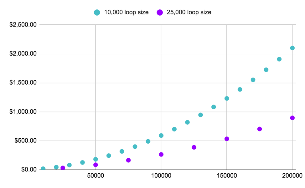
As seen on the graph below, it is easy to see how picking properly sized loops make a huge difference on the final compute bill. This is because smaller loops will clearly lead to additional retraining cycles, and because Active Learning usually assumes the model is to be retrained from scratch with all selected data at each loop. On the flip side, using larger loops make the selection process less precise, in that it is easier to miss “useless” data that could have been left out without any impact on model performance.
Figure 1: We show here the compute costs to train ResNet152 with 1.2M ImageNet records with two different Active Learning processes, both of which lead to the selection of 200,000 records (<20% of the entire dataset). While both processes would lead to the same savings in labeling costs, the process involving smaller loops (of size 10K) lead to a significantly more expensive compute bill. The only situation where it makes sense to choose the smaller loop size, is when the Active Learning process leads to better model performance.
TL; DR: It (quite literally) pays off to strategically tune the size of the loops to be used in the process.
By not retraining from scratch if possible
Active Learning can be a fantastic tool for ML experts (both to reduce cost and get higher model performance), but it is not without danger. A common pushback from Active Learning beginners is that actively selecting data can lead to biases, and this allegation isn’t without merit. Technically, Active Learning is meant to balance off model weaknesses by allowing the process to oversample with examples that appear to be difficult for the model to learn. So if it does what it is supposed to do, Active Learning should actually help improve representation and avoid that specific classes are overlooked by the model.
However, early loops can be tricky as selecting just a few corrupted examples could lead to situations that would be difficult to recover from. This is the reason why most practitioners prefer clearing their weights and starting from scratch with all selected data at each loop.
The inconvenience? If selecting 1,000 records at each loop, it would mean that by loop 5, we will have consumed as much compute as if we had trained on 15,000 records when having in reality only trained on 5,000 records at most. That’s 3x the amount of compute – and if your full dataset’s size was 10,000, you have already lost money compared to where you would be at without using Active Learning at all.
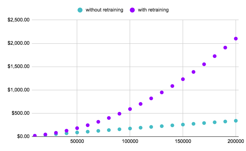
A new area of research lies ahead in deciding whether it is actually necessary to retrain on the full dataset, or if, instead, it would make sense to resume the training process with only the newly selected data. Furthermore, in later loops, it is even possible to consider using a form of Transfer Learning to save on compute. The following curve shows the ideal scenario where it could be avoided to retrain twice on the same data.
Figure 2: The plot above shows the difference in compute spent 1. when the weights of a deep learning model get cleared and the model is retrained on all selected data at each loop, and 2. when the model’s training process is only “resumed” with the additional selected data. There is a clear cost benefit to avoiding clearing the weights at every loop – but it is only advisable to do so if/when the model is stable enough to afford it.
TL; DR: Consider avoiding retraining later loops with the totality of selected data and decide instead not to clear the weights of a deep learning model once the model is stable enough.
By not computing inference for every single data point, at each loop
Vanilla Active Learning assumes that every unselected record that remains from the initial pool of raw data is to be considered for subsequent selection. That means that inference has to be run on every single remaining record, each time. For a million-record dataset seemingly performing well after 50,000 records have been selected, that’s a lot of inference (especially because it happens over and over again), and before you know it, the bill starts going up!
In order to avoid this type of situation, it can be wise to consider ways to reduce the scope of useful data. Researchers have successfully paired clustering with Active Learning in order to group unused records into groups of similar data and by only inferring on a fraction of each of the clusters. This is also where Information Theory can enhance the performance of your Active Learning process. An alternative approach is to infer on the same record with a lower periodicity (for example, each remaining record would only get inferred every 3 loops or so). Regardless of the solution you choose to adopt, this is a very important point to keep in mind if you are working with large datasets with a relatively low information density.
TL; DR: Inference calls can the demise of your Active Learning process. Learn to limit the number of inference calls if you are working with low-density, large datasets.
By distributing inference
Inference operations are commonly considered cost-efficient compared to training. However, the challenge in the case of Active Learning is that it relies on many iterative inference operations on potentially millions of records. Think that at each loop, it is normally expected that all unselected records (which in early loops would correspond to practically the entire dataset!) are put through inference, and that in this case, it is impossible to consider the compute due to inference as negligible compared to the compute due to training.
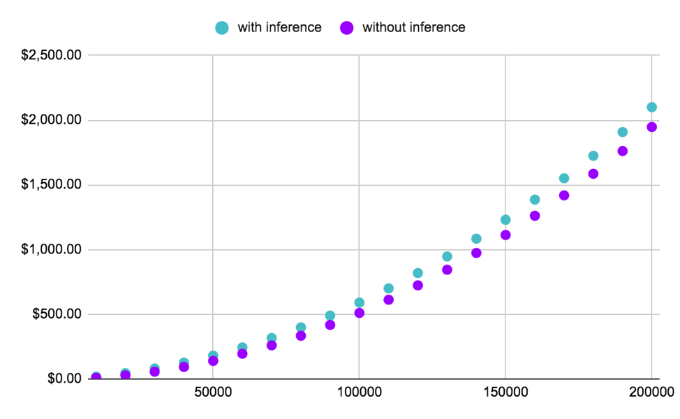
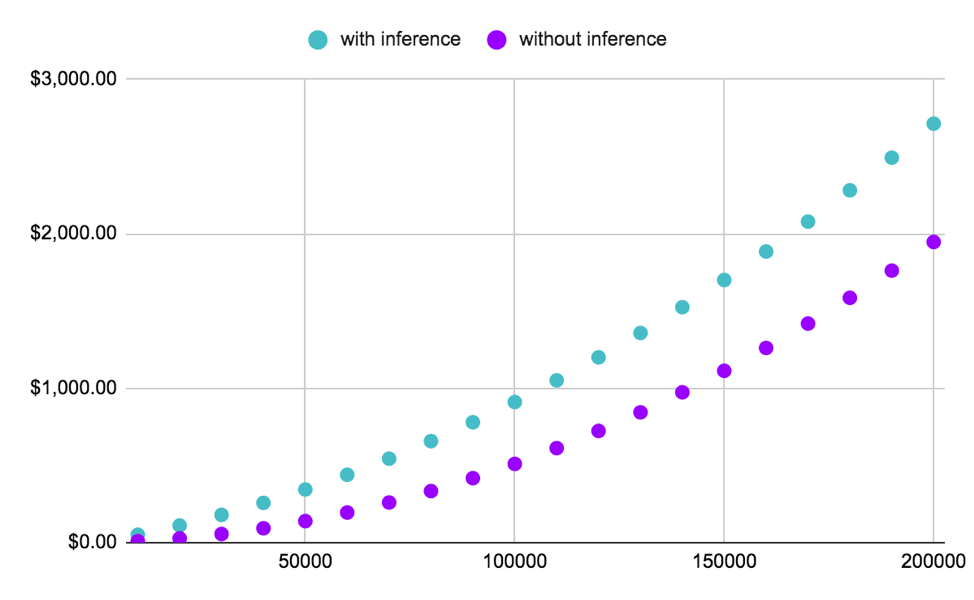
A solution to this problem is to rely on the relative ease of distributing inference jobs compared to distributing training. Alectio has recently started exploring a Distributed Active Learning workflow with its edge-compute partner, Distributive, where inference would be distributed and run on residual compute resources in a way that significant amounts of money can be saved on inference alone (specifically in cases where the cost of inference is not insignificant compared to the cost of training).
Figure 3: The plot shows how bringing the cost to inference to $0 would impact the total compute bill when running Active Learning on ImageNet / Resnet-152. The gain here is clearly not major.
Figure 4: On the other hand, this plot shows the elimination of the cost of inference when running Active Learning on SQuAD / BiDAF. This time, the total gain is very significant and justifies the trouble to use a distributed inference approach.
TL; DR: Run inference in a distributed manner on residual resources to minimize the costs associated with inference, so that you only have to worry about the cost of training.
The Active Learning Dream
After decades spent as a second class citizen in Machine Learning, it is a nice surprise to see such an increase of interest for Active Learning in recent times, and we can only hope and anticipate more exciting development in the field (from applications in ML Explainability to the more general adoption of Data-Centric AI).
However, a remaining barrier to the generalization of Active Learning workflows to all use cases and data types remains in the stigma associated to its computational inefficiency: if Active Learning does indeed deliver on its promise to save the user significant amounts of money on data labeling, it has historically not only failed to save money on compute, but has in practice increased the compute bills of the brave data scientists willing to give it a try. However, it is our undeterred belief that it would not take much to address the issue of compute-inefficient Active Learning and to develop and promote a new breed of Compute-Efficient Active Learning that would allow to save as much on compute as it does on annotation. And that is what would unquestionably lead, once and for all, to the general adoption of Active Learning by the ML community.


0 Comments